

Modeling Software Utilities
Complex Resistivity to Cole-Cole Inversion Program (CCINV)
CCINV inverts decoupled spectral complex resistivity data to Cole-Cole models with one to three additive Cole-Cole dispersions. CCINV allows inversion to either Cole-Cole or Zonge dispersion models. more
Station numbers represent distance along line, but may not be scaled to directly indicate length units. One to three dispersions may be used in the inversion model, although one is usually sufficient when using the Zonge model. Two Cole-Cole dispersions may be required to fit double-peak spectra, but the Zonge model can match double-peak spectra with a single dispersion. On rare occasions, it takes three Cole-Cole dispersions to fit some spectral curves.
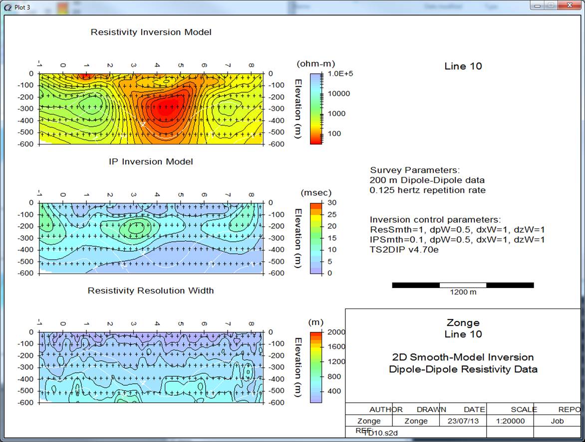 S2DPLOT image: 2D smooth-model inversion of dipole-dipole resistivity data showing both resistivity and IP plot panels
Color-Filled Contour Plots of 2D Resistivity/IP Inversion Results (S2DPLOT)
S2DPLOT reads Zonge TS2DIP inversion-program files (*.s2d, *.ipm and *.ipd) and creates multi-panel plots of inversion-model sections and data pseudosections.
Screen plots may be exported to the Windows Print Manager, to Windows metafiles (wmf), to portable network graphics (png) image files, to Surfer script and data files, or to Oasis montaj control and data files. more
Output files are given the same filename stem as the source inversion-model file, plus a plot number. By default, resistivity inversion results are shown on plot 1 and IP results on plot 2. Or resistivity and IP plot panels can be combined within a single plot.
Color-Filled Contour Plots of 2D CSAMT/AMT Inversion Results (SCSPLOT)
SCSPLOT reads Zonge SCS2D inversion-program files (*.mtm and *.mtd) and creates multi-panel plots of inversion-model sections and data pseudosections. Screen plots may be exported to the Windows Print Manager, to Windows metafiles (wmf), to portable network graphics (png) raster image files, to Surfer script and data files or to Oasis montaj control and data files. more
Output files are given the same filename stem as the source inversion model file, plus a suffix characterizing the plot number, 1 or 2. By default resistivity inversion results are shown on plot 1 and IP results on plot 2, but resistivity and IP plot panels can be combined within a single plot.
Color-Filled Contour Plots of Inversion Model Sections (MODSECT)
 At right: A MODSECT smooth-model inversion, resistivity cross-section of in-loop TEM data.
MODSECT reads Zonge inversion-program model files and creates color-filled contour plots of inversion-model-section resistivity or IP, one panel per plot. Plots may be viewed on screen or exported for hardcopy. more
- Reads scsinv m1d (CSAMT), steminv m1d (TEM), ts2dip IPM (resistivity/IP) or scs2d .mtm and .mtd (far-field CSAMT/natural-source AMT) files.
- Generates script and data files for use with Surfer v6 or v7.
- Exports GeoSoft Oasis montaj control and data files, which MODSECTGX.GX will turn into finished plots.
- Exports plots directly to the Windows Print Manager, Windows metafiles (wmf) or portable network graphics (png) raster files.
- Names output files with the same filename stem as the source inversion model file, plus a one-letter suffix: “r” for Resistivity section plot-file or “p” for IP model-section plot-file.
Interpolation to Plan-Map Data File (MAPDAT)
MAPDAT reads SCSINV and STEMINV *.M1D files, TS2DIP *.IPM or SCS2D *.MTM files, interpolates to a constant depth or elevation and then writes interpolated values to a tabular-format *.MAP file. *.MAP files have a simple spreadsheet format which can be used by Geosoft or Surfer. more
Making plan maps requires starting with a consistent grid coordinate system in *.STN files for each line, so that inversion results from multiple lines can be combined. Concatenate *.M1D, *.IPM or *.MTM files for a project area into a single large file. MAPDAT v3.01 can handle up to 16384 stations, ie 128 stations on 128 lines. Type “MAPDAT AUBELL.M1D” to extract an elevation or depth slice from AUBELL.M1D. MAPDAT will place the interpolated values into AUBELL.MAP. When you are generating multiple depth slices, you can rename the *.MAP file to something like ABZ500.DAT to avoid overwriting.
Note that S2DIP and SCS2D model sections extend past data coverage at each end of the survey line, but the model-section extensions are poorly resolved and may include spurious features. MAPDAT does not include automatic clipping on data coverage, so it is worthwhile to trim *.IPM and *.MTM model-sections back to the extent of data coverage before concatenating multiple lines into one large file.
You may select either constant elevation or constant depth slices in MAPDAT. You may also control the number of decimal places used in stations numbers. MAPDAT will read keywords from *.MDE files, parse keywords from the command line or will prompt you to enter values.
Utility Program for Skipping Noisy Data in TEM Sounding Curves (TEMTRIM)
Late-time TEM data are often corrupted by background electrical noise and noisy data points should be skipped before running data through inversion programs. TEMTRIM provides options for filtering TEM sounding curves, skipping noisy data, and/or integrating dB/dt(t) to calculate B(t) data. more
TEMTRIM reads TEMAVG *.avg files and writes updated *.avg and *.z files. The source *.avg file is saved with the extension *.av$. Using moving-average filtering modifies dB/dt values. Trimming noisy late-time segments does not modify or delete data, but sets skip flags. Calculating B(t) adds a column of data to the *.avg file and a block of data to the *.z file. TEMTRIM v3.10 is a MS Windows program using ‘high-color’ or ’16-bit’ color graphics.